“Hmmm, this is about one of those mysterious magnetic antennas!”
The “hairpin” monopole antenna has been around for a long time. During this time numerous questions have been raised concerning its performance, namely ” How can a balanced structure radiate?” and “What is its impedance?” This article will attempt to answer these questions. A hairpin monopole is simply one half of a folded dipole, therefore, a good starting point for our discussion is to briefly describe the electrical properties of the folded dipole antenna.
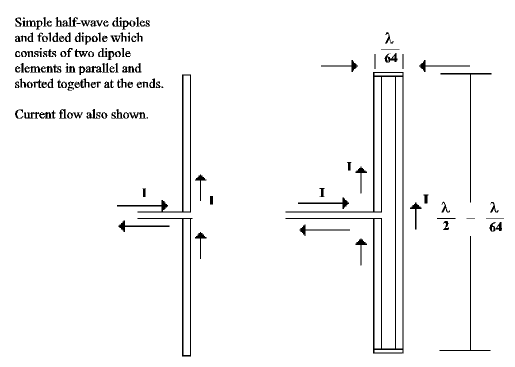
A folded dipole antenna is a center-fed half wave dipole with another half-wave element close to it and joined at the ends as shown in Figure 1. The spacing between the elements is about 1/64 wavelength and the overall length approximately one-half wavelength. Electrically, a dipole antenna can be expressed as a series resonant circuit consisting of a resistive component and two reactive components. At the resonant frequency, the impedance which results from this combination becomes resistive because at resonance the reactive components are of equal and opposite characteristics and cancel each other. The resultant resistance is 73.16 ohms for a vanishingly thin dipole.
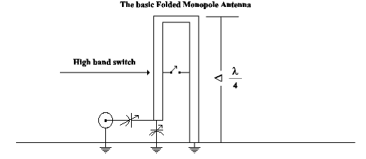
The Hairpin Monopole Antenna - Figure 1
Typically, because of finite physical dimensions, a 1/2-wave dipole antenna will exhibit a resistance of about 68 ohms depending upon its length to diameter ratio.
A folded dipole, in addition to the series resonant circuit, has a parallel resonant circuit. The parallel resonant circuit is the result of the two elements being shorted together at the far ends. The shorted ends hold the voltage at these two points to the same value: therefore the distribution of voltages and currents for the two elements remains the same as it would for a simple dipole. When the two elements of the folded dipole are of the same diameter, the input resistance becomes four times that of a simple dipole. Theoretically, 4 x 73.16 = 293 ohms (less in practice). This is the reason why a 300-ohm twin lead transmission line is used with folded dipoles.
The increase in resistance at the feedpoint point comes about because there is an equal division of the current in the two parallel elements. Since there is a division of current at the feedpoint, there is only one-half the current at the feed point that there would be for a simple dipole. Thus, for the same amount of power fed to the antenna (or received by the antenna) only half the current appears at the feedpoint and the resistance is increased by 4. This is more readily understood by examination of the basic equation:
R = P/I2 ohms (1)
Halving the current (I) but keeping power (P) constant means that, when the 1/2 value of current is squared, its final value in the equation will be only one-forth the value had it not been squared:
R = P/[I/2]2 = P/[I2 /4] 4P/ I2 = 300 ohms (2)
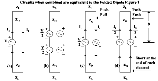
One may wonder, how can a folded dipole, which appears to be a short-circuited balanced transmission line radiate? Balanced lines are not supposed to radiate. The folded dipole is basically an unbalanced (and therefore radiating) transmission line. To see this, let us assume that a transmission line, consisting of two parallel conductors, is fed in the center of one side but not the other side, Se Figure 2(a) and 2(b). This constitutes an unbalanced condition. as we shall soon see. To find the currents and impedance presented to the generator, the unbalanced source is replaced by a pair of equivalent sources, one in the push-push configuration, Figure 2(d), and one in the push-pull configuration as shown in Figure 2(c).
The Hairpin Monopole Antenna - Figure 2
Now for the Maths
The push-push configuration will first be considered. For simplicity, let the far end impedance be replaced by ZL. These impedances transform along the line so that at the generator they have a value which we shall call Z1, that is:
ZI = ZO [ZL + ZO tan q/ ZO + ZL tan q] (3)
Where:
ZO = Impedance of parallel lines
ZL= Impedance of termination
q= half length of parallel lines in electrical degrees.
Z1 = Impedance seen by generator
For the short-circuited condition where ZL=O, Equation (3) simplifies to:
ZI = ZO tan q (4)
It follows that the transmission-line current is:
It = V/2Z1 (5)
In the push-push configuration, Figure 2(d), the voltage sources are in parallel. With this type of arrangement, no current flows through the loads ZL and the antenna current is:
Ia = V/2Za(6)
When we look at the balanced and unbalanced parts, it becomes clear that the currents are not equal. The current in the left side of the line is:
Ileft = It + Ia/2 (7)
while that in the right side is:
Iright = It– Ia/2 (8)
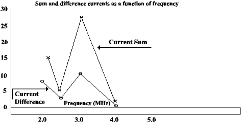
Figure 3 illustrates graphically the sum and the difference currents as a function of frequency for a hairpin monopole antenna.
The Hairpin Monopole Antenna - Figure 3
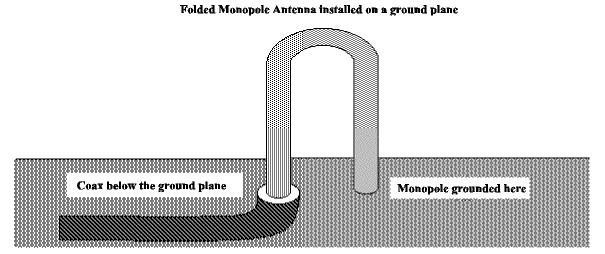
One-half of a folded dipole antenna can be operated above a ground plane so as to function as a folded monopole type of antenna. This is the basic structure of the hairpin monopole antenna. Under these conditions, for a perfectly conducting ground plane, the input impedance is one half that of a half-wave folded dipole, about 150 ohms.
Figure 4 illustrates the basic folded monopole or hairpin antenna. The noted difference between a basic folded monopole antenna and a hairpin is that the hairpin is considerably shorter. Shortening an antenna reduced the radiation resistance. General Dynamics developed a 10(c) kW hairpin antenna only 14 feet high that tuned the 2 to 30-MHz range in two bands: 2 to 8 MHz and 8 to 30 MHz.
The Hairpin Monopole Antenna - Figure 4
The General Dynamics hairpin antenna uses a short-circuiting switch part ways up the antenna to modify the impedance of the antenna while operating in the high band. The switch serves to reduce the length of the transmission line for the transmission line currents and maintains the desired inductive reactance properties of the antenna. This short-circuiting switch does not affect the radiation currents or radiating pattern of the antenna. The radiation pattern is essentially omnidirectional in the horizontal plane. An inductively reactive antenna can be tuned or matched with variable capacitors as shown in Figure 5.
The Hairpin Monopole Antenna - Figure 5
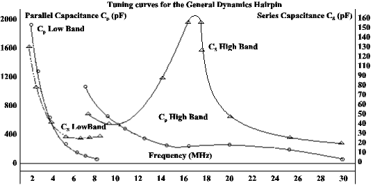
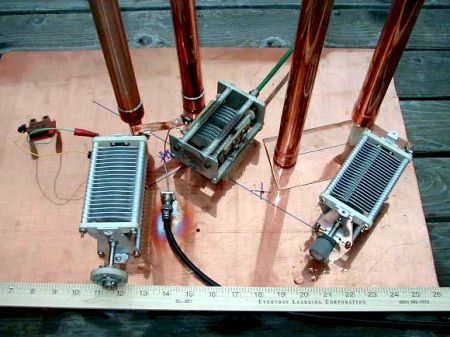
The high power requirements of the General Dynamics hairpin antenna requires the use of special tuning capacitors. Capacitors with a 1000-pF, 500-ampere, 45 kV ratings are mandatory. Figure 6 presents tuning curves for the shunt capacitor (Cp) and the series capacitor (Cs) for the General Dynamics hairpin monopole antenna.
The Hairpin Monopole Antenna - Figure 6
Tests run on the hairpin indicate that a “tuned up” Standing wave ratio of less than 1.3:1 can be achieved using this matching technique.
Editors Comments
The article on the Hairpin Monopole is representative of a magnetic antenna, of the same type as the DDRR. I hope someone will use the information found in this very interesting article and build a hairpin monopole. The following formulas will help anyone build a hairpin:
Height = 28/F (in MHz)
Spacing between conductors = Height/28
The results are in feet and in the case of the spacing between the conductors, in percentages of a foot. For an example, a 160 meter hairpin will be computed this way:
Height = 28/1.8 = 15.56 ft. and the spacing = 15.56/28 = .57 ft. or a fraction over 6 inches between radiators.
The tuning capacitors, CP, the parallel capacitor should be a 2000 pF, capable of standing high voltages. The value of CS, the series capacitor should be 150 pF, also with high voltage capabilities. These values come off of the charts in the article.
It should be apparent from the chart on radiation resistance that large conductors need to be used to reduce the losses from skin effect to as low a value as possible. This is very important, and is a factor that is often overlooked in the construction of this type of antenna. A GOOD ground is extremely important!
It is also interesting to note that a 10 meter version is only one foot tall with a spacing of only .035 ft.(.42 inch) and CP is about 55 pF and CS is about 22 pF. That wouldn’t take too much copper pipe, and it would be easy to build and tune.
A version for CB would only be one foot and a half inch tall, and the spacing would be not quite 1/2 inch. By using a 5 watt CB transmitter, the voltage requirements for the tuning capacitors would be reduced. It is certainly somewhere to start.
Again it is important to state that all joints need to be soldered, not bolted together or pop riveted. The resistance of such a connection would far exceed the radiation resistance of the antenna. So solder all joints, and use copper tubing, the larger diameter the better. Automotive tail pipe tubing and other large diameter conductors like down spout tubing have too high skin resistance due to the material that is used in their construction. Copper is the cheapest thing we can get for this type of project.
There is a definite need for more experimentation with this kind of antenna. As hams we can exercise our talents experimenting with this kind of antenna. For the unfortunate soul that is in an antenna restricted area, this might be an answer.
Originally posted on the AntennaX Online Magazine by Wilfred Caron
One Month Later...
Condensed Information
The Hairpin Monopole Antenna - Figure 1
We have had a lot of questions on the hairpin monopole antenna. Here is some quick and useful information for those who are sort of overwhelmed by the math in the article by Wilfred Caron previously published by antenneX..
The formula 28/f is correct for this antenna, and the rest of the information on the last page of the article is correct for building an antenna for any frequency. Keep in mind that the capacitors will have to handle a lot of current and voltage for typical amateur power levels, in the 100-200 watt level. It will also have a very narrow frequency range before retuning will be required.
Grounding requirements are both a ground rod and radials, since a copper ground sheet is out of the question for most of us. Capacitor sizes are 160 pF for the series capacitor and 2000 for the parallel capacitor
Ham band dimensions and how they were derived
160 meters, 28/f=15.56 ft. (4.73 m) = Height 15.56/28=6.84 in (17.37 cm) = Spacing
Conversions for Other Bands
Band
Height
Spacing
80 m
7.46 ft – 2.269 m
3.197″ – 8.12 cm
40 m
3.88 ft – 1.18 m
1.65″ – 4.2 cm
30 m
2.77 ft – 84.2 cm
1.18″ – 2.99 cm
20 m
59.9 ft – 59.9 cm
0.84″ – 2.13 cm
17 m
1.54 ft – 46.9 cm
0.66″ – 1.67 cm
15 m
1.3 ft – 40 cm
0.55″ – 1.4 cm
12 m
1.12 ft – 34 cm
0.48″ – 1.21 cm
10 m
11.8″ – 29.94 cm
0.42″ – 1.06 cm
These figures are for the middle of each band, and should allow coverage of the entire band, with the possible exception of the two lower bands, 160 and 80 meters. This is only speculation and is an unknown as far as amateur usage is concerned.
Construction should be with all soldered connections and the usage of copper tubing of at least 1 inch is advised. No pop rivets, no bolted connections and connections held with hose clamps. This is due to the extremely high currents that will flow in this type of antenna. For the effort to build one, construction of a loop will give better results and greater bandwidth. However, for those who wish to experiment with this antenna, the figures are here. Also some sort of fence should be constructed around the antenna, if it is going to be at ground level, to keep people or animals away from the antenna when it is being used. Again, this is due to the high voltages present on the antenna.
If you do decide to make one of these antennas, keep your power down and you will be able to use normal tuning capacitors, instead of vacuum variables. This is also a problem with all types of magnetic antennas. There will be a lot of hams interested in the results that anyone gets with one of these antennas. Let us know if you do build one of these antennas and your results will be published here.
Originally posted on the AntennaX Online Magazine by Richard Morrow, K5CNF
Part 2 - Lab Notes of the Hairpin Experiments
Last month (December 2000 issue of antenneX) I described some experiments using a short “Hairpin Antenna” at 20 meters and the results of coupling it with a second version in a parasitic mode to broaden its bandwidth. This month the addition of a series-tuned circuit was tried as a “trap” to provide a “short” part way up the antenna to tune it to resonance at a higher frequency with the same settings that resonate the Hairpin at the lower frequency. Along the way I discovered a very useful interactive Smith Chart tool that helps greatly in understanding matching calculations.
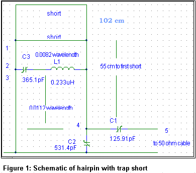
John A Kuecken’s book of 1969 (“Antennas and Transmission lines”, page 225) shows how the unsymmetrical currents generated by feeding one side of a shorted balanced transmission line are the means of radiating energy in a hairpin antenna. He also states that these currents pass by a short that is switched in on his antenna to allow tuning at a higher frequency band. He said the entire antenna length radiates at the higher band. Accordingly, I modified the antenna used last month by replacing the short at the top that was made with two right angle pipe fittings with a short made with two “tee” fittings connected together. The rest of the available copper pipe was then used to extend the hairpin from about 53 cm height to 1.5 meters. The original short was then placed on top of the extended antenna. This, then, simulated the antenna in its “high band” mode.
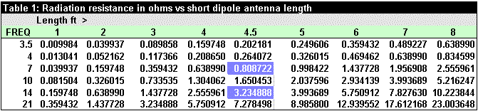
The first step was to get some idea of the expected radiation resistance of a short antenna versus frequency and length. Table 1 shows the radiation resistance of a short dipole with constant current throughout its length, which is electrically much shorter than a wavelength. The achieved value will be less than half these values for a monopole with non-constant current. The Table shows that a dipole antenna 4.5 feet long has a radiation resistance of about 0.8 ohms at 7 MHz and about 3.2 ohms at 14 MHz.
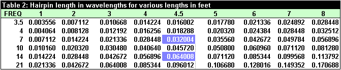
Table 2 shows the length in wavelengths at various lengths and frequencies. Figure 1 shows the schematic of the extended Hairpin antenna with a shorting trap part way up the first section. It can be seen that the trap shorted Hairpin antenna is a complex microwave circuit involving radiation resistance, L,C, and transmission line components. A perfect problem application for the Smith Chart!! In casting about for a Smith Chart program to solve this problem, I came upon a Smith Chart site! The reader may enjoy loading up the website and using the tools described while reading this experiment.
This site has many references, and includes a real treasure: the Motorola Interactive Matching Program. It is specialized for matching a source to a load, such as two amplifier stages, or an amplifier to an antenna. Download it!! It’s free! It allows the user to pick up to 11 frequencies, and then asks for the load impedance (in this case the radiation resistance in ohms with no reactance) and source impedance (in this case 50 ohms). Then it provides a page where one can construct the network beginning at the load. The antenna book mentioned above suggested that the antenna matches the radiation resistance to the cable impedance, so I defined the load as the radiation resistance.
Table 1 has the values used indicated by a colored cell. Then the MIMP program lets the real fun begin! The Smith Chart is presented and one can switch a window to any component to adjust its value while watching the Smith Chart change. The first thing to do is adjust the normalization to 50 ohms, which means that the center point on the chart represents the desired output of 50 ohms pure resistance. I set it up with 5 frequencies between 7 and 7.2 MHz and 5 between 14 and 14.2 MHz. The Smith Chart shows two little arcs of 5 “x”es, one for each frequency, and a group for the impedance seen looking toward the load from each numbered point in Figure 1. The desired load of 50 ohms can be surrounded by a circle representing all points around 50 ohms that result in a specified return loss. Return loss is the number of decibels down from the incident power that equals the reflection from the (slightly) mismatched load. As one adjusts some parameter, say the series capacitor to the output, the little groups of “x”es sweep around the Smith Chart. The object is to make them both (7 and 14 MHz groups of 5) arrive at the center, within the circle of 20 dB return loss.
Like Flying Spaceships
Using the MIMP is like flying a group of spaceships around some universe near earth, which is represented by the 20 dB return loss circle. As a component is adjusted to scan the output arcs past the resonant point, or point of closest approach to “earth”, an intuitive appreciation of the Smith Chart and the network workings develops! It is harder to explain than to do!
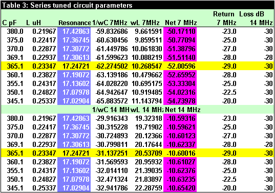
Table 3 shows the return loss as the tuning is changed while watching 7.15 and 14.15 MHz. The values of the L and C in the trap series tuned circuit are shown, along with the resonant frequency of the tuned circuit. It is evident that it is not working as I first envisioned: the tuned circuit is not shorting the hairpin transmission line at 14 MHz. Instead, the net capacitance after adding the L and C reactances is combining with the delay line length in wavelengths. The net reactance and each component reactance are shown.
Table 4 shows the transformed impedance at each of the numbered points in Figure 1 for all 10 frequencies, looking toward the load. The Table illustrates how each component changes the transformed impedance, until the required matched load is neared by the arc of “x”es at 5. Table 5 gives the measured lengths of the antenna.
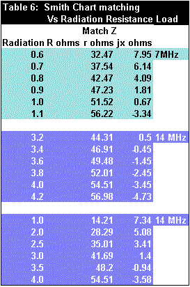
The results were not as good as I expected. While it tuned up easily at 7 MHz, the 14 MHz resonance gave a best SWR of 6 to 1. All the components were adjusted around their design setting with no improvement. Apparently the problem was the uncontrolled one, the radiation resistance, which was much too low to transform to 50 ohms. Table 6 shows the matching at 7.15 and 14.15 MHz as radiation resistance is varied. The transformed radiation resistance moves up toward 50 ohms with only a small reactance term as radiation resistance increases.
But it’s doing what it should
It wasn’t until I was writing this and checking the numbers in the tables that it was realized that, as usual, the experiment was doing exactly what it was designed to do – not what I thought it was doing. Table 1 is the radiation resistance for a DIPOLE, and the hairpin is a MONOPOLE, which will have half the radiation resistance. Or less if the current is not constant along its length!! The experiment corrects the thought processes in the endless iteration toward perfection!!!
The New Hairpin Experiment
It looks like extending the antenna about a meter will make it work. Next month I will do that and also test the effects of adjusting the height of the 2-inch gap between the driven side and ground – which is the a-symmetry that produces the radiating current in the hairpin. I am also curious what happens if the top is open rather than shorted.
Originally posted on the AntennaX Online Magazine by Joel C. Hungerford, KB1EGI