I Want to Build a 3 Element Yagi - Part 1 - How Big Shall I Make It?
Those of us with more time than money get the urge to upgrade our antennas from dipoles to beams in the home workshop. The logical first step might be a 2-element Yagi. Often, we skip this step because we have heard or seen evidence that 2-element Yagis do not quite have the specifications we want. If we decide to use the common reflector-driver design, the gain is low and the front-to-back ratio is poor. If we opt for a driver-director design, we get more gain and better front-to-back ratio, but a very narrow beamwidth and a potentially very low feedpoint impedance. So we immediately jump to 3-element designs.
Our next step is usually a semi-fatal one. We search the magazines and handbooks on our shelves for a design that looks like one we can build. We know what the author claims the beam will do, but we are not ever sure of how it does what it is supposed to do or whether our version is doing the same thing.
So let’s back up a bit and look at some 3-element Yagi basics. I shall focus on monoband beams, because they are much easier than multi-band beams to model and to build so that their performance matches the model. Even if you have your heart set on buying a tribander, perhaps these basics will help you better to understand both the antenna maker’s claims and the performance you actually get.
The basics I have in mind have little to do with the theory of parasitic element operation. The ARRL Antenna Book and some references I shall mention along the way do a good job at that level of explanation. Instead, I shall begin in the middle of things with some distinctions among Yagi designs. There are so many Yagi designs floating around today that they can be at first sight a bit bewildering.
High Performance Design
The first decision we have to make is whether we wish to have a wide-band Yagi or a high-performance Yagi. Let’s begin with the high-performance designs, since these have very great initial appeal. We shall return later to some wide-band designs.
Once we have opted for a high-performance design, we have to figure out what we mean by that term. First, there is the matter of size. The element lengths will not vary by a large amount from one design to another (but they will vary significantly in terms of the performance). So, size turns out to be a question of boom length.
James Lawson, W2PV, developed most fully the notion that the gain of a Yagi is highly dependent upon the boom length. His book, Yagi Antenna Design, has become one of the classic references for those interested in basic Yagi theory. Based on his work, many designers have optimized 3-element Yagis of various lengths for maximum performance.
Maximum performance is a balanced mix of high gain, good front-to-back performance, and a satisfactory feedpoint impedance. Let’s work backwards through the list.
For almost any length boom, one can get a little more gain from a Yagi by so spacing and sizing the elements that the feedpoint impedance drops to about 10 Ohms or less. Most high performance designs you will encounter tend to opt for feedpoint impedances closer to 25 Ohms. The reasons are many, but one good reason is a matter of losses. Suppose that the total resistance of all the connections at the feedpoint, including those of a matching system for 50-Ohm coaxial cable, amount to 1 Ohm. (That is a quite high value and can be reduced by good construction practices.) With a 10-Ohm feedpoint impedance, about 9-10% of the power is going to heat. If the feedpoint impedance is 25 Ohms, then the loss is closer to 4%.
To this consideration, we can add the fact that it is generally easier to design low-loss matching systems for a 25-to-50 Ohm conversion than for a 10-to-50 Ohm conversion. So 25 Ohms becomes a kind of de facto (but not absolute) limit to a Yagi’s feedpoint impedance.
For the higher feedpoint impedance, it is also somewhat easier to design a 3-element Yagi whose gain and front-to-back performance figures hold up across such HF bands as 20 and 15 meters–as well as the first MHz of 10 meters. As well, the designs can be replicated in the home shop with moderate building skills and are not so finicky as to require industrial laser measuring equipment in setting the dimensions.
Within these constraints, then, lets look at three good designs for 3- element Yagis.

As revealed in Figure 1, the designs I have in mind use three different boom lengths. The long-boom design, shown for 28-29 MHz, is adapted from an optimized design by K6STI. It uses an 11.31′ boom, which is nearly 1/3 wl long. The K9EUV design uses a 9.88′ boom, and has the additional feature of using equal spacing between elements. (A fourth director element at the same spacing and the same length as the present director provides good 4- element Yagi performance.) The third design is a short boom Yagi, also by K6STI, that requires a 7.5′ boom. For construction, you should round these boom-length numbers upward to the next whole foot to provide room for mounting plates and hardware. So we have 12, 10, and 8 foot boom 3-element Yagis.
Caution: Do NOT build these designs as given here. They all use uniform diameter elements. Converting them to the actual lengths needed by physical designs that employ tubing that decreases in diameter will net us different dimensions. But that is a subject for a future episode.
The 10-meter designs all use 0.5″ aluminum tubing. We can scale them for any band in the following way. Take the ratio of the new design frequency (for example 14.175 or 21.22 MHz) to the present design frequency (28.5 MHz) and invert it (since lower frequencies will require longer, fatter elements). Now multiply the element lengths, the element spacings, and the element diameters by this figure.
As a sample, here is a collection of dimensions for the three basic designs for 10, 15, and 20 meter versions of the antenna.
Long Boom
Frequency
28.5 MHz
21.22 MHz
14.175 MHz
Element Lengths
Reflector
Driver
Director
17.90 ft
16.41 ft
15.44 ft
23.11 ft
22.06 ft
20.76 ft
34.56 ft
33.00 ft
31.05 ft
Spacing
Reflector-Driver
Driver-Director
5.20 ft
6.01 ft
6.99 ft
8.08 ft
10.46 ft
12.09 ft
Element Diameter
0.5 inches
0.75 inches
1.0 inches
Medium Boom
Frequency
28.5 MHz
21.22 MHz
14.175 MHz
Element Lengths
Reflector
Driver
Director
17.27 ft
16.63 ft
15.62 ft
23.20 ft
22.34 ft
20.99 ft
34.72 ft
33.43 ft
31.41 ft
Spacing
Reflector-Driver
Driver-Director
4.94 ft
4.94 ft
6.63 ft
6.63 ft
9.92 ft
9.92 ft
Element Diameter
0.5 inches
0.75 inches
1.0 inches
Short Boom
Frequency
28.5 MHz
21.22 MHz
14.175 MHz
Element Lengths
Reflector
Driver
Director
17.65 ft
16.15 ft
15.41 ft
23.75 ft
21.71 ft
20.71 ft
35.50 ft
32.47 ft
30.98 ft
Spacing
Reflector-Driver
Driver-Director
3.00 ft
4.50 ft
4.03 ft
6.05 ft
6.03 ft
9.05 ft
Clearly, I have violated my own scaling scheme by using the closest standard value of aluminum tubing as the element diameter. Hence, some very small adjustments are required in the element lengths and spacings, but generally, these are too small to make an operational difference. Nonetheless, some of the difference shows up numerically in the design frequency performance figures for the three designs. Here the table divides the designs by bands.
20 Meters : 14.175 MHz Antenna Design
Long Boom
Medium Boom
Short Boom
Free Space
Gain (dBi)
8.11
7.78
7.13
Front to Back
(dB)
27.31
35.50
41.35
Feed Impedance
R +/- jX Ohms
25.71 – j 0.93
27.02 + j 0.50
27.46 + j 0.01
15 Meters : 21.22 MHz Antenna Design
Long Boom
Medium Boom
Short Boom
Free Space
Gain (dBi)
8.16
7.81
7.17
Front to Back
(dB)
26.12
34.88
61.67
Feed Impedance
R +/- jX Ohms
24.80 + j 0.37
26.06 + j 0.94
26.56 + j 0.00
10 Meters : 28.50 MHz Antenna Design
Long Boom
Medium Boom
Short Boom
Free Space
Gain (dBi)
8.11
7.08
7.12
Front to Back
(dB)
27.15
34.77
41.66
Feed Impedance
R +/- jX Ohms
25.70 + j 0.80
26.51 + j 1.69
27.45 + j 0.01
These tables of predicted performance from NEC models show a number of things, including how to be misled. First, the numbers–even though slightly different in the decimal columns–illustrate that for each design, the performance is identical on all three bands. The excess decimals are given because NEC reports them and because they show how little different the performance varies as we correctly scale a beam from one band to another.
However, the front-to-back figures can mislead us into thinking that the short-boom model has an almost miraculously better front-to-back performance than the other beams, as good as they are. The figure given is for the 180-degree front-to-back ratio, which is usually a very convenient figure to obtain. That figure may not be indicative of the performance of the antenna in all its rearward directions.
Figure 2 provides an overlay of the 28.5 MHz free space azimuth patterns of all three antenna designs. We may note the forward gain peaks, which just about correlate to the differentials in boom length. The rear lobes give us much more valuable information. Here we see that the long-boom design has three small lobes of roughly equal size so that the front-to-back ratio in the table gives a fair appraisal of the overall front-to-rear performance. In contrast, the other two models have deeper 180-degree “dimples,” combined with much stronger angling lobes. When averaged out, none of the antennas has much of an advantage over the other. Indeed, anything above 20-dB front-to-back ratio overall might be considered outstanding.
To this point, it may seem that the decision we need to make is one of gain advantage vs. mechanical disadvantage to a longer boom. However, let us not be so swift to judgment. For I have once more misled you by giving you the peak or nearly peak performance of the antenna at one frequency. The next question is how each of these designs performs across an entire ham band.
Since the first MHz of 10 meters is the greatest stretch for these designs (because 20 and 15 are proportionately narrower), let’s sweep the antennas across the 28 to 29 MHz range and see how the performance of each holds up.
In Figure 3, we have the gain of the three designs across the pass band. Note that the gain figures in the tables are intermediate values. The gain across the band can vary by as much as 0.4 dB in at least one of the designs. In selecting a design, we must also ask whether the lowest gain–which occurs at the low end of the band for 3-element Yagi designs–is an acceptable figure (when weighed against all of the other factors involved in our decision to build).
Figure 4 records the 180-degree front-to-back ratios across the pass band. Here we can either be impressed by the peak values, or we can take a closer look at the values at the band edges. The short-boom design actually excels in this department, with no value falling below 20 dB. The other two designs are remarkably close in their band edge values, which are about 17 dB at the low end and 15-16 dB at the high end. Before settling on a design for the two lower bands, we should remember that these bands are only 68% to 70% as wide as the 10-meter passband. Hence, we can achieve better band-edge results by centering the peaks in our final design.
A rough measure of whether we shall be able to effect a wide-band match to a 50-Ohm cable can be derived from the SWR curve of the antenna related to the resonant impedance before matching. Since the feedpoint impedance of all three models is so close to 25 Ohms, we can use that number as representative of the resonant feedpoint impedance. Then we can evaluate the SWR curves in Figure 5.
For all three designs, the SWR climb more quickly above the resonant design frequency than below it. On 10 meters, this means exceeding a 2:1 SWR value at the upper end of the pass band for two of the three designs. However, all three designs will likely show under 2:1 SWR across the narrower reaches of 20 and 15 meters. The short boom design shows the flattest curve.
Although the designs were set up for a resonant feedpoint impedance (little or no reactance), one can extend or shrink the driver length as necessary to use any of the common matching system: beta, gamma, Tee. Of course, a 1/4 wl section of 35-37 Ohm coax will provide a matching section to a 50-Ohm main line if we leave the feedpoints resonant. We shall look in more detail at typical matching systems before we are done.
So it looks like we are almost ready to make a decision. Seemingly, all we need to do is to look at how the elements might change if we use several diameters of tubing for each one.
Not so fast. We have not yet looked at truly wide-band designs to see if they hold any advantages and what those advantages might be. So while we are still in this preliminary stage of design evaluation, let’s look next month at a pair of wide-band Yagi designs.
I Want to Build a 3 Element Yagi - Part 2 - How Wide-Band Shall I Make It?
Last time, we looked at the basic design of high-performance 3-element Yagis. All had similar front-to-back and feedpoint impedance characteristics. They differed in gain in accord with the length of their booms. For 10-meter models, here are the design center figures as a reference for this month’s investigation:
10 Meters : 28.50 MHz Antenna Design
Long Boom
Medium Boom
Short Boom
Free Space
Gain (dBi)
8.11
7.08
7.12
Front to Back
(dB)
27.15
34.77
41.66
Feed Impedance
R +/- jX Ohms
25.70 + j 0.80
26.51 + j 1.69
27.45 + j 0.01
Each of these designs is capable of performance close to that at the design frequency across the first MHz of 10 meters. When scaled to 20 and 15 meters, the designs will cover the entire bands–and, of course, cover the WARC bands when scaled to those frequencies.
However, there is an alternative design philosophy. This philosophy sacrifices some gain in favor of wide-band characteristics. For example, the high-performance models might vary in gain by almost 0.5 dB across the span from 28 to 29 MHz. A wide-band design might vary in gain across the same span by only 0.15 dB. Likewise, a high-performance design with a feedpoint impedance in the mid-20s might just barely allow a 2:1 SWR at the band edges. A wide-band design might show those figures over the entire 10-meter band, with a corresponding shallow SWR curve within the first MHz of 10 meters.
Consequently, before we freeze our design decisions, let’s look at the basic wide-band 3-element Yagi design a little more closely.
Wide Band 3 Element Yagi Design
To create a wide-band 3-element Yagi requires more boom length for a given gain than used in the high-performance designs we surveyed last time. A 12′ boom on 10 meters will yield about 1 dB less gain. What, then, is the rationale for such a design?
The fundamental reasons for going to a wide-band design are two:
1. The wide-band design provides reasonably smooth and quite adequate performance figures for the entire 10-meter band, which is 1.7 MHz wide. Hence, a single beam will cover the CW/SSB and the FM/satellite portions of the band. When scaled to 20 or 15 meters, the beam will show less change in gain, front-to-back ratio, and feedpoint impedance across those bands.
2. The wide-band design can be set for a feedpoint impedance very close to 50 Ohms, thus eliminating the need for any sort of matching network at the feedpoint. (However, a choke or 1:1 choke balun remains recommended to attenuate common mode currents.)
When these two reasons are combined, the result is a very close match to a standard 50-Ohm coaxial cable feedline with very small changes in SWR across the band of choice. This eases not only matching problems, but as well the sensitivity of some transmitting equipment to even low SWR levels that often result in automated power output reductions. Accompanying this feature is consistent gain and front-to-back ratio performance across the band.
There is an additional feature occasionally anecdotally noted by some operators. They claim superior performance results from Yagis with higher input impedances. Since these claims do not show themselves in NEC models, the vehicle we are using to evaluate performance potential, no comment can be made upon those experiences in this context.
Since the performance of wide-band models shows up most clearly on 10-meter models, we shall focus solely upon them. You can extrapolate the most relevant portions of performance curves for the other HF bands.
Two notable designs for wide-band 3-element Yagis have appeared in US antenna literature in the last decade. In the May, 1990, issue of Ham Radio, Bill Orr, W6SAI presented a wide-band design in one of his columns. In the Winter, 1998, issue of Communications Quarterly, Joe Reisert, W1JR, presented a similar design, along with scaleable design equations.
Figure 6 shows schematically both the Orr and the Reisert designs, set for 10 meters. As we noted in connection with the high-performance designs, do NOT commit to using these dimensions to construct either design. Both are predicated on uniform diameter elements: 0.5″ for the Reisert design, 1.0″ for the Orr design. In common practice, Yagi elements consist of two or more sections of tubing each side of center, each section having a smaller diameter than the preceding one. This tapered-diameter schedule results in a need to lengthen elements relative to uniform-diameter models. We shall explore this topic next time.
For the moment, we want to look at the wide-band designs as concepts rather than as finished products. Both the designs require 12′ booms (with allowance at each end for element-mounting hardware). The dimensions of the two antennas are sufficiently close to each other that we suspect similar performance will emerge from the antennas. And we get it.
The free-space azimuth patterns in Figure 7 overlay the Orr and Reisert designs at their resonant frequencies. The differences are too small to require comment. Gain is within 0.02 dB; front-to-back difference is less than 1 dB; and the feed point impedances are within 1 Ohm of each other at resonance. For reference, here is a handy table of values:
| Antenna | Resonant Frequency (MHz) | Free Space Gain (dBi) | Front to Back dB | Feed Impedance R +/- jX Ohms |
|---|---|---|---|---|
| Orr, 1990 | 28.80 | 7.11 | 21.60 | 47.08 + j 0.98 |
| Reisert, 1998 | 28.85 | 7.13 | 20.92 | 46.01 + j 0.20 |
The slight differential in resonant frequency owes to the slight design differences, which in turn yield slightly different performance curves on 10 meters. Moving the resonant point allows one to obtain a satisfactory SWR curve across the band. We can easily sample the performance by running frequency sweeps. In the following graphs, I have used 29.5 MHz as an arbitrary upper limit in order to limit the number of data points.
The free-space gain figures for the two designs appear in Figure 8. The Reisert model shows the smoother gain curve, although the differences are marginal. Note that in wide-band designs, there is often a dip in the gain at the low end of the band. The dip reaches minimum for the Orr design below the lower end of 10 meters.
If we translate the first MHz of the band into roughly equivalent performance across 20 or 15 meters, the Reisert design, especially, shows a very small change in gain. The consistency of performance across the band is one of the advantages of a wide-band design.
What the Orr design gives up in gain, it reacquires in front-to-back performance, as shown in Figure 9. If we use a 20-dB front-to-back ratio as a plateau figure of merit, then the Orr design would show this across all of 20 and 15 meters. However, the Reisert design averages only about 1 dB less performance in this category, an amount unlikely to be either noticed or measurable.
With either design, the 180-degree front-to-back ratio used in the graph is a reasonable approximation of overall front-to-rear performance. The smooth rear quadrant lobe shown earlier in the azimuth patterns ensures a reasonable correlation between the 180-degree front-to-back ratio and the other two common measure of rearward performance: an averaged front-to- rear ratio and a worst-case front-to-back performance figure.
Where the wide-band designs shine is in the flatness of the SWR curves. As shown in Figure 10, the 50-Ohm SWR curves for both designs permit a ready match directly to 50-Ohm feedline across 10 meters. If the curve centers are translated into equivalent 20 and 15 meter versions, achieving a maximum band-edge SWR of 1.35:1 is no real challenge.
For those willing to accept a slightly lower gain on the HF band of choice, the wide-band design offers consistent performance across the band with an ease of matching to 50-Ohm feedlines systems that the high-performance models cannot duplicate. The wide-band models, however, offer only the gain that the high-performance models achieve with a boom 2/3 as long.
Before we close out this preliminary survey of designs, let’s take a moment to review what we are seeking to do when we decide that we want to build a 3-element Yagi.
A Pair of 2-Element Yagi Designs
Although we can design a 2-element driver-director Yagi of excellent performance and very compact size for the WARC bands, covering the wider HF bands requires that we look to 2-element driver-reflector designs. In order to see just why we might want a 3-element version, let’s look at two versions of the 2-element Yagi. One uses narrow spacing, the other wide spacing.
Figure 11 shows the dimensions of both models, which use 1″ uniform diameter elements. In these very standard designs, the element lengths are quite similar, with only small changes needed to accommodate the difference in boom length. At the design frequency of 28.5 MHz, the short boom is just under 1/8 wavelength long, while the long boom is somewhat over 1/6 wavelength long. At the design frequency, the modeled performance characteristics are these:
| Antenna | Frequency (MHz) | Free Space Gain (dBi) | Front to Back (dB) | Feed Impedance R +/- jX Ohms |
|---|---|---|---|---|
| Narrow Space | 28.50 | 6.27 | 11.24 | 32.65 – j 0.32 |
| Wide Space | 28.50 | 6.13 | 10.65 | 51.71 + j 9.23 |
As the table makes clear, the design frequency gain is about 1 dB less than that of the wide-band 3-element Yagi and 2 dB less than the 12′ boom high- performance version.
The gain curve in Figure 12 shows that, contrary to the curves for Yagis with a director, the gain for a driver-reflector Yagi descends as the frequency increases. Were we inclined to mislead you, we might do one of two things. First, we might suggest–based on the gain value for ONLY the low end of 10 meters–that there is little difference in performance between 2- and 3-element Yagis, using either the short boom high-performance or the wide-band 3-element Yagi as a comparator. Second, using ONLY the gain value for the high end of the pass band graphed in the figure, we might try to convince you that a 3-element Yagi has an inordinately high gain advantage over the 2-element version. Both claims would be equally inaccurate. Only a graph of values over a relevant frequency range tells a full story.
With respect to the 2 2-element designs, the narrow-spaced version has the higher gain across the pass band. For this exercise, only the first MHz of 10 meters is shown, although the wide-spaced version will be usable across the entire 10-meter band.
The overall front-to-back ratio of a 2-element driver-reflector Yagi is fairly weak, failing to reach 12 dB as shown in Figure 13. (Note: this weaker front-to-back ratio can be an advantage in certain kinds of net and contest operations where total exclusion of signals from the rear quadrants can be a hindrance to efficient operation.) The narrow-spaced version has the stronger values, but the curve is clearly sharper than the gentler slope of the values for the wide-spaced version. The wide-spaced model front-to-back ratio is about 10 dB at the upper limit of the 10-meter band.

The SWR curves in Figure 14 for the two models tell different stories. The sharp curve for the narrow-spaced model has a resonant point of about 32.5 Ohms. Hence, the antenna will require a matching network for a 50-Ohm main feedline. In contrast, the curve for the wide-spaced model is based on 50 Ohms. The curve has been intentionally shifted downward in frequency to show the shallow rise in value above the lowest value. By moving the center point of the curve upward in frequency simply by shortening the driver element slightly, the SWR can be held below 2:1 across the entire 10-meter band. This permits direct matching to a coax line with no matching network needed (but with the recommended choke or choke balun in place, as always).
With the 2-element Yagi curves in mind, we can make more precise our reasons for wanting to move to a 3-element Yagi.
1. Most prominently, for operations that need it, the front-to-back values for all versions of the 3-element Yagi are considerably superior to those of the 2-element driver-reflector Yagi.
2. The gain of a high-performance, long-boom 3-element Yagi show about a 2 dB advantage over the 2-element Yagis. This amount of gain is significant. The short-boom and the wide-band 3-element Yagis show about half that value of extra gain, and the significance of the difference is reduced accordingly.
3. Both 2- and 3-element Yagis can be designed for 50-Ohm feedpoint impedances that hold up even across the wide reaches of 10-meters. However, in both 2- and 3-element designs, narrower spacing allows more gain per unit-length of boom.
Figure 15 shows comparative free-space azimuth patterns for the narrow-spaced 2-element Yagi, the wide-band 3-element Yagi, and the 12′ boom high-performance Yagi. The steps of performance improvement are clear in the graphic. What the patterns cannot show is that, where narrower band operation and a 25-Ohm feedpoint impedance are acceptable, the short-boom 3-element Yagi will provide roughly the same gain and front-to-back ratio as the wide-band model with 2/3 the boom length.
In the end, the final decision as to which design meets our needs will use some mixture of the performance figures, plus a measure of the physical properties of the structure we propose to build. Hence, every such decision will be very individualized. The various models we have presented are intended only to provide some comparative measures as a background against which to make the final decision.
Still, we have not addressed some of the structural considerations that go into the decision. Boom length so far is a matter of a number, not a real physical property. As well, we need to look at what real tapered-diameter elements may imply for the antenna design. Both of these questions mean that we shall have to add a “Part 3” to this series–next time.
I Want to Build a 3 Element Yagi - Part 3 - What Real Dimensions Shall I Use?
Had the 3-element Yagis we explored in the first two parts of this investigation been designed for VHF, we might have been able to use the dimensions as given. At VHF and above, we often use elements with uniform diameters. However, at HF, the most common practice is to use elements composed of tubing whose diameter decreases as we move outward from the element center. That makes a big difference–perhaps the difference between a beam that works and one that only seems to work.
Tapered-Diameter Elements
The relationship between uniform-diameter and tapered-diameter elements has long been guessed at, but only in the last decade or two has it been fully appreciated. Perhaps the most complete treatment of that relationship appears in David Leeson, W6QHS, Physical Design of Yagi Antennas. Leeson’s conversion equations are built into some antenna modeling software (EZNEC and NEC-Win Plus).
When an element in the vicinity of 1/2 wavelength long is composed of materials which taper downward in diameter away from the center point, the required length for resonance increases relative to an element of equivalent uniform diameter. Moreover, the equivalent uniform diameter is not simply the average diameter of the materials used.
Figure 16 gives us some examples to explore. Each shows 1/2 of a resonant aluminum element for 28.5 MHz. At the top, the element is roughly equally divided. The second element uses the same sequence of tubing, but in unequal lengths. The bottom element uses the same inner section lengths as the first example, but with a steeper taper.
In this example, and in all element-diameter taper schedules, only the exposed part of each tubing size is shown. Where one tube fits inside another, an additional overlap length of about 3″ is generally recommended. Anything more tends to add weight without adding strength, and much less than the 3″ overlap may jeopardize junction strength.
The examples show that the required length for resonance changes if we change the relative lengths for a given taper schedule or if we change the taper schedule itself. The following table can make the changes even clearer.
| Example (Figure 16) | Required Length (inches) | Average Diameter (inches) | Equivalent Diameter (inches) | Length of each Equivalent Element (inches) | Feed ZR +/- jX |
|---|---|---|---|---|---|
| Top | 100.8 | 0.623 | 0.631 | 98.58 | 71.8 – j 0.1 |
| Middle | 100.6 | 0.634 | 0.598 | 98.67 | 71.8 – j 0.1 |
| Bottom | 102.4 | 0.742 | 0.739 | 98.39 | 71.8 – j 0.2 |
The more radical the taper, the longer the required length for resonance. Variable length sections alter the length and the equivalent uniform diameter. Sometimes the equivalent diameter is close to the average–and sometimes not.
Many home Yagi builders tend to freely substitute materials in a design, unconcerned about the changes in element length that may be required to get the same performance as the original. These same builders often lack any means of checking performance other than an SWR meter. Hence, they assumed that if the antenna has the same feedpoint characteristics as the original, it must yield the same performance. The assumption is very often a bad one.
Without sophisticated antenna test range equipment, the best method available to check a Yagi without any element loading for performance is antenna modeling software. Both MININEC and NEC (the latter with tapered- diameter corrections built in) have been calibrated and tested extensively, and Yagi designs that pass the modeling test generally perform as modeled. There are almost always slight variations between the model and the physical version of the antenna, but in most cases, they are far smaller and less detrimental to performance than the guess work that marked the first 30 years of home Yagi design after World War II.
Let’s look at some dimensions for 3-element monoband Yagis using various diameter taper schedules for 10, 15, and 20 meters. The differences from our uniform-diameter study models may be instructive. The following notes will use common US aluminum tubing sizes, which tend to come in 1/8″ increments. A common wall size of 0.58″ permits succeeding tube sizes to mate closely and still have enough play to slide one within another with ease. Since builders in other parts of the world must work with available sizes, usually specified in millimeters, here is a small table of equivalences.
| US Size in inches | Size in mm | US Size in inches | Size in mm |
|---|---|---|---|
| 0.375 | 9.5 | 1.000 | 25.4 |
| 0.500 | 12.7 | 1.125 | 28.6 |
| 0.625 | 15.9 | 1.250 | 31.8 |
| 0.750 | 19.1 | 1.500 | 38.1 |
| 0.875 | 22.2 | 2.000 | 50.8 |
Because non-US antenna elements will likely have a different set of element diameter transitions, it is especially important to remodel a Yagi design when changing the element dimensions from English to metric.
Some 10 Meter Designs
We shall look at only two of the many possible element taper schedules one might use for 10-meter beams. See Figure 17.
Following the work of K6STI, we shall call the upper schedule the high- loading schedule, because it was thought to be better able to withstand higher winds. The lower version is called the medium wind load schedule. Other schedules are not only possible, but are in use by both home builders and commercial manufacturers. Some beam-makers prefer heavier, more rigid element designs, while others prefer more “aggressive” tapers that flex without breaking. End diameters of 7/16″ and 3/8″ are used in some commercial designs. A builder who wishes to depart from one of the “ordinary” element designs may wish to consult a computer program called YagiStress to check the survivability potential of a proposed element diameter schedule.
As a consequence of the many possible element designs, we can only sample a couple, with the goal of ultimately comparing tapered element lengths to the uniform lengths used in our initial look at different Yagi design philosophies. Our point will be, in part, to verify that the performance promised by the uniform-diameter designs can be obtained with tapered elements.
10 meters is a good starting point, because the diameter changes in a given element are the fewest. Let’s begin by comparing the dimensions of our short boom study design with version built from the taper schedules shown in Figure 17. Dimensions will be in inches. The “end” section length will simply be the difference of half the total length and the distance from element center up to the start of the last tubing section.
| Antenna Dimensions | Uniform Diameter (0.5″) | High Load | Medium Load |
|---|---|---|---|
| Reflector Length | 211.8 | 216.0 | 215.0 |
| Reflector -DE Space | 36.0 | 36.0 | 36.0 |
| DE Length | 193.8 | 203.6 | 202.0 |
| DE-Director Space | 54.0 | 54.0 | 54.0 |
| Director Length | 184.9 | 189.0 | 187.2 |
All of these antennas use the same element spacing. The parasitical element dimension extension of the tapered-element designs runs from 3 to 5 inches, but the driven element required for resonance is 8 to 10 inches longer than the uniform element.
One evidence that the antennas are comparable is the feedpoint impedance (R +/- jX Ohms) at 28, 28.5, and 29 MHz.
| Frequency (MHz) | Uniform-Dia (0.5″) | High Load | Medium Load |
|---|---|---|---|
| 28.0 | 27.0 – j 11.5 | 28.8 – j 11.0 | 30.0 – j 10.6 |
| 28.5 | 27.5 – j 0.0 | 28.9 – j 0.3 | 30.1 + j 0.2 |
| 29.0 | 22.6 + j 14.0 | 23.5 + j 13.6 | 24.7 + j 13.9 |
We can make a similar comparison between the uniform-diameter wide-band Yagi and a tapered version. Let’s use the Reisert design, along with a “high-load” tapered version of the same antenna.
| Antenna Dimensions | Uniform-Dia (0.5″) | High Load |
|---|---|---|
| Reflector Length | 211.8 | 214.8 |
| Reflector -DE Space | 69.2 | 70.0 |
| DE Length | 193.8 | 199.2 |
| DE-Director Length | 63.8 | 63.0 |
| Director Length | 177.8 | 184.8 |
In this case, we have made some slight but important changes in the element spacing to achieve performance across the entire 10-meter band, mainly in centering the front-to-back curve so that performance at the band edges is comparable. Both the original and the tapered version of the antenna provide under 2:1 50-Ohm SWR across the band. However, the dimensions of the tapered version differ significantly from the uniform-diameter version. Thus, even if a designer provides neat equations for calculating uniform- diameter elements, those equations disappear from utility once one moves to tapered-diameter elements.
To establish that the modified beams perform like the originals, let’s look at a pair of graphs.
Figure 18 provides gain curves from 28 to 29 MHz for all 5 Yagis in the tables above. The gain values for the high-performance, short boom models are within a few hundredths of a dB of each other. The difference between the tapered and untapered wide-band Yagis averages under 0.1 dB.
The front-to-back curves in Figure 19 tell a very similar story. All three of the high-performance, short boom Yagis show the same high mid-band peak in 180-degree front-to-back ratio, with similar passband edge performance. The wide-band models show insignificant differences and also end up at very similar values at the wider band edges of the design. In short, with some care in adjusting element lengths–and occasionally the element spacing– one can achieve the same basic performance from a tapered-diameter Yagi as from a uniform-diameter version of the same design.
Some 15 Meter Designs
In Figure 20, we can examine the differences between high-load and medium- load element tapers for 15 meters.
Obviously, each level requires an additional, larger tubing segment to accommodate the longer element. Corresponding design dimensions for the original uniform-tape design and tapered-diameter designs appear in the following table.
| Antenna Dimensions | Uniform-Dia (0.75″) | High Load | Medium Load |
|---|---|---|---|
| Reflector Length | 284.4 | 289.0 | 286.0 |
| Reflector -DE Space | 48.4 | 48.0 | 48.0 |
| DE Length | 260.5 | 274.0 | 271.0 |
| DE-Director Space | 72.6 | 92.0 | 92.0 |
| Director Length | 248.5 | 254.0 | 251.0 |
The difference in overall boom length is immediately noticeable–a matter of 19″ or over 10% of the total length. In some respects, the tapered- element beams are not the same design as the study model, although the longer elements required by element-diameter tapering are apparent. The 15-meter study model was scaled directly from the 10-meter model, while the taper-diameter models came from work by K6STI.
One consequence of the longer boom with about the same reflector-driven element spacing is a lower feedpoint impedance. The following table shows the difference:
| Frequency (MHz) | Uniform-Dia (0.75″) | High Load | Medium Load |
|---|---|---|---|
| 21.0 | 27.4 – j 6.2 | 20.5 – j 9.2 | 21.4 – j 9.9 |
| 21.225 | 26.6 – j 0.0 | 20.4 + j 1.0 | 22.1 + j 0.3 |
| 21.45 | 23.5 + j 9.0 | 20.7 + j 10.0 | 22.5 + j 9.4 |
The shorter, uniform-diameter model would permit more versatility in matching and would likely be amenable even to a 35-Ohm 1/4 wl matching section. The lower impedances of the longer tapered-diameter models would likely require a beta match or similar, with suitable adjustments to the length of the driven element.
However, there may be compensation for the lower source impedance.
The gain curves in Figure 21 show the nearly half dB gain advantage accrued from using a longer boom. Not only is the gain higher, but it changes less across the 15-meter band.
In Figure 22, we discover that all three models have excellent front-to-back ratios, never worse than 20 dB. Since the peak value reflects a deep dimple in the rearward lobes, differences have less importance: roughly equally high marks go to all three designs.
In the end, the decision comes down to whether the lower feedpoint impedance and the 19″ of additional boom are worth the added gain. The shorter length boom with tapered elements can be developed into a beam having characteristics very close to the study model–as we saw in the case of 10-meter beams.
Some 20 Meter Designs
Tapered element design can become quite complex as we move to the 20-meter band. See Figure 23.
The medium load element adds one more section to the corresponding 15-meter element. However, the high-load model adds two sections. In addition, the 1/4″ jump in diameter as we enter the center section of the element generally suggests that two tubing sections of the same length are used: a 1.125″ diameter section inside the 1.25″ section.
Once more, if we turn to our short-boom model, we obtain dimensions of the following values.
| Antenna Dimensions | Uniform-Dia (1.0″) | High Load | Medium Load |
|---|---|---|---|
| Reflector Length | 425.9 | 447.3 | 438.0 |
| Reflector -DE Space | 72.4 | 80.0 | 90.0 |
| DE Length | 389.6 | 421.6 | 414.0 |
| DE Director Space | 108.6 | 106.0 | 106.0 |
| Director Length | 371.7 | 393.3 | 386.0 |
Despite the use of larger diameter sections in each element, the high-load element has the more radical taper and results in a greater required element length at each position than the thinner but less radically tapered medium-load element. The element position adjustments, necessary to sustain performance across the 20-meter band, elevate the source impedance from about 25 Ohms to about 30 Ohms.
A similar significant lengthening occurs with the long-boom (24′) high performance Yagi design.
| Antenna Dimensions | Uniform-Dia (1.0″) | High Load |
|---|---|---|
| Reflector Length | 414.7 | 433.8 |
| Reflector -DE Space | 125.5 | 125.5 |
| DE Length | 396.0 | 415.0 |
| DE-Director Space | 145.1 | 145.1 |
| Director Length | 372.6 | 391.0 |
Note that the boom length is here preserved. The average element length increase is about 19″ for the radically tapered high-load element or nearly 5% of the total element length.
The gain curves in Figure 24 show that for each type of beam, we obtain similar gain curves relative to untapered and tapered models.
In Figure 25, we can see the front-to-back performance. The two high- performance models have values that closely overlap. The short-boom models place their front-to-back peaks at different frequencies. If the high-load model peak were moved upward in frequency by just a bit, its band-edge performance would closely parallel the other two models.
Some Miscellany
The point of our exercises has been to familiarize you with the effects of element-diameter tapering on overall Yagi dimensions. Moving from a uniform-diameter design to one that includes multiple tubing sizes requires careful redesign to take into account the actual element-diameter taper used. This is no casual design process, but rather a task of optimizing dimensions throughout the design. Programs such as YO and YagiMax can mechanize the process to a great degree.
The particular models used in this exercise do not mean that any particular design is recommended. However, the range of models does suggest a set of standards, relative to performance expectations and boom length.
Several items have not be covered. For example, the models surveyed so far all assume insulated mounting relative to the boom. We have not looked at the so-called “plumber’s delight” element mounting system. One technique for dealing with the effects of direct electrical mounting to the boom is to create a short, large-diameter wire at the very center of the element.
Also missing is a consideration of the requirements and the hazards of long booms. When viewed from the mast-to-boom mounting assembly, the boom is a pair of lever arms. The longer the arm, the greater force exerted by an element of some preset size. Seemingly small increases in boom length can require close attention to boom strength. The increase in boom length can also create larger wind forces as viewed from mast. Nonetheless, very durable assemblies have been created for Yagis far larger then our 3-element models.
Although the high number of variables involved in the physical structure of 3-element Yagis would make a short discussion less than useful, there is a subject to which we might devote one more part in this series: feeding and matching the antenna to a standard 50-Ohm coaxial cable feedline.
I Want to Build a 3 Element Yagi - Part 4 - How Shall I Feed the Antenna?
Because our purpose has been to look at the basic electronic design aspects of the 3-element Yagi, we have omitted structural details. We shall also bypass matters of supporting and rotating the antenna, even though they involve some interesting facets of horizontal antenna performance at various heights above ground. Most of these items are relevant to almost any horizontal antenna, and we wish to remain focused on the 3-element monoband Yagi.
One detail that we dare not overlook is the method of feeding the Yagi. Actually, the term “feeding” is a bit of a misnomer, since it involves the establishment of an impedance match between the antenna and the main feedline. We shall assume that the main feedline is a standard 50-Ohm coaxial cable. (You may, of course, feed the Yagi with any parallel feedline, using an antenna tuner at the shack end of the line. This would permit use of the antenna on many bands, although directional characteristics would be optimal on only one band. However, some remnant directivity may exist on bands adjacent to the one for which the Yagi is designed.)
Feeding the wide-band designs is simplicity itself. To attenuate common mode currents, a choke or 1:1 choke balun is recommended at the antenna feedpoint. Designs ranging from 1:1 toroidal baluns to ferrite-bead baluns to a coil of coax sized for the band in use appear in the standard references, such as the ARRL Antenna Book.
Feeding the high-performance beams we have surveyed is another matter entirely. For these designs, the antenna feedpoint impedance ranged from 20 to 30 Ohms. All of the driven elements were set to resonance, but we can make any adjustments necessitated by the type of matching system we use. Changing the length of a driver by 2 to 3% makes no operational difference in the antenna performance, although it may change the resistive component of feedpoint impedance by a few Ohms. However, it will be the change in the reactive component of the feedpoint impedance that will be most critical to adjusting the matching system.
One common criticism of using matching networks with Yagis is that they introduce losses. However, calculations show that with reasonable care in design, these losses no where exceed 2% of the applied power, a loss of only about 0.08 dB. By contrast, most 3-element Yagi designs that do not need a matching network have gains that are near to or exceed 1 dB lower than those of the high-performance designs. Hence, the use of a matching system should not be considered a negative aspect of a design, so long as the feedpoint impedance does not go too low. Good construction and maintenance practice is, of course, assumed in this note.
Tees and Gammas
Two related forms of feeding a Yagi and at the same time elevating the feedpoint impedance to 50 Ohms are the Tee and the Gamma. (The “Tee” is actually named the “T” for its shape, but adding the “ee” ensures that the single letter is not missed by the reader.) Both methods of feed permit the direct physical and electrical connection of the driven element to the boom.
As Figure. 26 shows, we make our feedline connection to a rod or double rod that parallels the element for a distance, at which point we connect a shorting strap to the rod and the element. The gamma match permits a direct conversion of the antenna feedpoint impedance to 50 Ohms. In the gamma match, the coax braid is connected directly to the electrical center of the element.
The Tee double rod system is most effective in raising the impedance to a much higher value than 50 Ohms. 200 Ohms is a convenient value, since a 4:1 balun then provides a fine 50-Ohm match, while performing the task of attenuating common mode currents at the same time.
In VHF beams, many builders have noted and measured some pattern distortion with the gamma match. Hence, the Tee has almost become a standard for beams having other than a 50-Ohm feedpoint impedance. HF beam makers have more confidence in the gamma match, whose parts are a relatively smaller proportion of the driver structure than they are at VHF and UHF. However, the Tee is inherently balanced.
The dimensions of both matching systems depend upon the relative sizes of and the spacing between the element and the rod material. Calculations are best done with software specifically designed for the task. YO (Yagi Optimizer), by K6STI, for example, has such auxiliary software, and independent utility calculation programs are available as freeware from many sources.
Note that the sketches in Figure 26 did not include a series capacitor at the feedpoint and rod junction, a standard feature in many basic system sketches. In most instances, variable capacitors do not withstand well the rigors of weather. Moreover, the reactance of the system can be set (or nulled, depending upon one’s perspective) by adjusting the length of the driven element.
The Beta Match
If you are willing to use a driven element that is insulated from the boom, matching networks become very much simplified. Let’s begin with the beta match. Many hams distrust the beta match because the small “hairpin they see across the feedpoint looks like a short circuit. They just do not understand how the beta match works.

In Figure 27, we see a common L-network to match a source impedance that is high to a load impedance that is lower. One way to accomplish this is to place a shunt (or parallel) inductor across the source and add a series capacitor to the load. The network arrangement assumes that both the source and the load impedance are purely resistive.
The equations for calculating the proper values for an L-network are very simple. First, let’s calculate delta, a figure of “merit” (sometimes called network Q) for the proposed network. For this purpose, we can use the equation
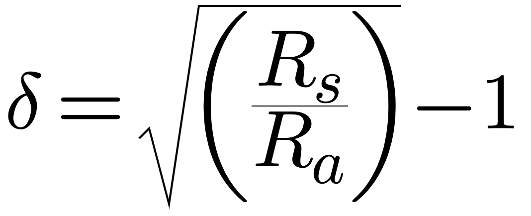
where Rs is the source resistive impedance and Ra is the load resistive impedance. As noted., Rs is higher than Ra. From delta and the values for Rs and Ra, we can calculate the reactances of the shunt and series components of the network:
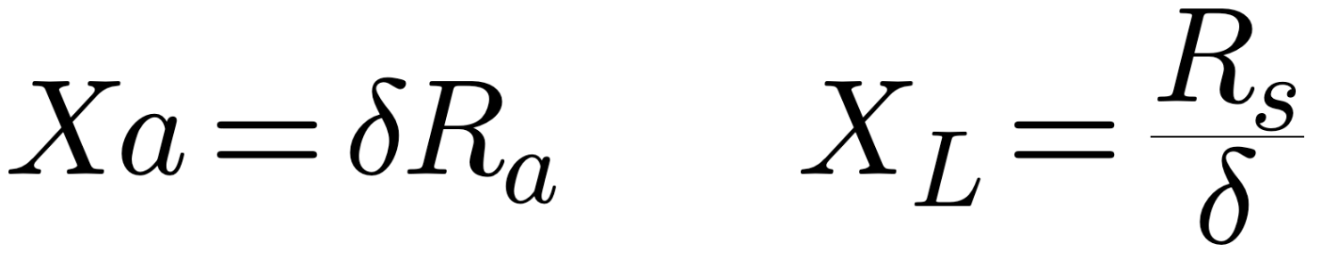
Xa, the series reactance, can be converted into a value of capacitance for the design frequency, although we shall not have to do this in our application. The value designated as Xl gives the reactance the shunt component. In principle, we can use a series inductor and a parallel capacitor as easily as we might use as series capacitor and a shunt inductor. In most, but not all, antenna applications, the series capacitive reactance and shunt inductive reactance is more usual–and is most apt to our 3-element high-performance Yagi designs.
As the lower part of Figure 27 indicates, we can obtain the series capacitive reactance without using a separate capacitor. We simply shorten the driven element which changes the resonant resistive feedpoint impedance to a complex value having a capacitive reactance component. How much do we shorten the element?
The answer to this question has two parts. First, we need to know what amount of series capacitive reactance we need. If we assume that Rs is 50 Ohms, the characteristic impedance of our main feedline and the transmitter connected to it, then we can calculate the required value of both the series and the shunt reactances. Since all of our beams had feedpoint impedances between 20 and 30 Ohms, we can reduce the problem to a little chart.
| Load Resistance Ra (Ohms) | Source Resistance, Rs=50 Ohms 30 | Source Resistance, Rs=50 Ohms 25 | Source Resistance, Rs=50 Ohms 20 |
|---|---|---|---|
| Delta | 0.817 | 1.0 | 1.225 |
| Series Xa (Ohms) | 24.5 | 25 | 24.5 |
| Shunt Xl (Ohms) | 61.2 | 50.0 | 40.8 |
The chart tells us several things, including the answer to the second part of our question about the series capacitive reactance. We need to shorten the driven element by an amount that will yield a series capacitive reactance that is near to 25 Ohms. For a 20-meter driven element using aluminum tubing, the overall shortening of the element will be about 10″ or so. On 10 meters, half the shortening will yield about the same capacitive reactance at the feedpoint. Shortening the element by this much may lower the resistive component of the feedpoint impedance by an Ohm or perhaps two, but, as you can see from the chart, the required series capacitive reactance will not change by a significant amount.
The value that changes most with changes in the resistive component of the feedpoint impedance is the shunt inductive reactance necessary to effect the match to the 50-Ohm source.
We can provide a shunt inductive reactance in two normal ways. We can convert the inductive reactance for the design frequency into a value of inductance using standard handbook equations. Then we can design a simple coil (a single layer solenoid, as it is called) of #14 to #10 wire having the right inductance. For the small values involved, it is fairly easy to design an inductor with a Q between 200 and 300. Since the network losses are roughly (but not exactly) equal to the value of delta divided by the coil Q, we can see that in ordinary circumstances, losses will be under 1%. Moreover, we can adjust the precise inductance of the small coil by spreading or squeezing the turns until the 50-Ohm SWR at the network terminals is 1:1.
An alternative to the inductor is the shorted transmission line stub. For the most compact assembly and widest bandwidth, a wide-spaced “hairpin” made of wire or rod creates a shorted parallel transmission line section with a high characteristic impedance. The required length is a function of the wire diameter, the spacing, the frequency, and the required reactance. Handbook equations can be used for this calculation, although independent utility software exists to combine all of the calculations into one exercise. One such program was created by WA1SPI and is included in the HAMCALC collection available from VE3ERP.
Although some builders prefer to have an adjustable shorting bar as the rear part of the hairpin, my own preference is for a single hairpin with longer legs. We adjust the hairpin length by clamping down at the antenna feedpoint on the legs at the right points. This system reduces the number of mechanical connections by 2, which in turn reduces the number of potential resistive loss points.
The hairpin tends not to answer directly to standard Q formulations, since it changes the value of reactance in a manner different from the way in which coils change reactance values as we move off the design frequency. However, a hairpin with a characteristic impedance above 600 Ohms tends to have a similar bandwidth characteristic to a beta coil with a Q of 300 or more.
Figure 29 shows the 50-Ohm SWR values across 20 meters for one of our 3- element models set up with a beta match consisting of a 600-Ohm shorted transmission line a little over 11″ long. Modeling software does not show transmission line losses, but parallel lines that are about 1/70 of a wavelength do not have much loss when composed of wires or rods sufficiently thick to handle the currents involved.
One caution is necessary with beta matches. It is possible to find a setting for a coil or a hairpin that effects a match when the series capacitive reactance is not optimal. Often, these settings result in additional and unnecessary losses from the network. Hence, it is important that the builder set the driven element as close as possible to the correct length for the required value of capacitive reactance at the feedpoint.
The Quarter Wavelength Matching Section
For designs that have a resonant feedpoint impedance close to 25 Ohms, we can use the driven element as given and effect a match to a 50-Ohm line in another way: the 1/4 wavelength matching section.
In Figure 30, we can see the simplicity of the system. Although 35-Ohm transmission line runs about $3 a foot, it provides a set-and-forget matching system (except, of course, at our semi-annual inspection and maintenance sessions).
The use of 35-Ohm cable for the matching section is based on the standard impedance transformation effects of 1/4 wavelength transmission line sections, which answer to the equations
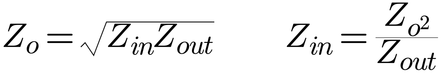
where Zo is the characteristic impedance of the matching system, Zin is one of the two resistive impedance values being matched, and Zout is the other value being matched. The 1/4 wave line length, of curse, is the electrical length, and the physical length must be adjusted for the velocity factor of the line–which yields for all coaxial lines a physical length that is shorter than the electrical length. In many cases, the 1/4 wavelength section can be coiled to act as a common mode current choke while still performing its matching duties.
The losses of a 1/4 wavelength matching section will be as low as those of any other matching system. Programs such as N6BV’s TLA can be used to check line losses both at the resonant frequency and at the band edges, using projected feedpoint impedance values supplied by an antenna modeling program.
As shown in Figure 31, a quarter-wavelength matching section is capable of performance very similar to a beta match when it comes to 50-Ohm SWR values across 20 meters. The values in Fig. 31 are insignificantly different from those recorded in Figure 29.
However, the two methods of impedance transformation are sufficiently different to yield actual impedance values that are also different, despite the fact that the values result in quite similar SWR values. The following table shows the modeled feedpoint impedance values for the same Yagi model with a beta match in one instance and with a quarter-wavelength matching section in the other.
Matching                      Source Impedance (R +/- jX Ohms)
System              14.0                14.175              14.35
Beta                79.6 + j 11.3       50.9 - j  2.7       27.9 - j  0.5
     50-Ohm SWR          1.65                1.06                1.79
1/4 WL Section      35.8 + j 17.8       47.6 + j  1.7       39.5 - j 22.9
     50-Ohm SWR          1.70                1.06                1.75
Conclusions (Of a Sort)
In the end, the selection of a Matching system for a high-performance 3- element Yagi with a feedpoint impedance in the 20-30-Ohm range will depend on a number of factors outside the limits of electrical design. First, the selection of construction design will limit the matching network options. Direct connection of the driven element to the boom will eliminate both the beta and the quarter-wavelength matching systems. The Tee can be used with insulated or uninsulated drivers (relative to the boom). In general, most but not all commercial designs have gravitated toward the used of drivers that are insulated from the boom. In fact, a number of available designs insulate all elements from the boom.
If cost is a factor, the beta match using either a home-made hairpin or coil is likely the cheapest matching system available–but it is no less effective for its low cost. (Although the hairpin is about as cheap as you can get, it is no license to skimp on the quality of hardware used anywhere in the beam. Low quality hardware tends to result in both mechanical and electrical problems with any beam antenna.)
The beta is also fairly easy to adjust, since it is located very close to the hub of the antenna boom-to-mast region. Hence, readjustment at the tower top is easier than with Tees or Gammas. Often, settings chosen in near-ground preliminary assembly phases hold good at the final antenna height.
This entire series has been devoted to some of the electrical design options available to the builder of his or her first 3-element Yagi. A Yagi of this size and performance makes an excellent project for the home builder, since most of the materials can be obtained with reasonable ease. Multi-band Yagis, on the other hand, are best left for later exercises, once one has become thoroughly familiar with all of the parameters of Yagi design–or they are best left to the professional designers who can spend 8 hours or more each day on this difficult task.
If you have never used an antenna as good as a 3-element monoband Yagi, you are in for some real surprises and adventures in operating–once you complete the project. Where your dream designs take you after that will be your own responsibility.
Originally posted on the AntennaX Online Magazine by L. B. Cebik, W4RNL
Last Updated : 4th May 2024