
The Crossed Field Antenna - Part 1
Preface
Please be aware this article introduces a completely new concept in antenna theory. In fact, this is considered the most important development relative to antennas in this century. It is so pervasive that a series of articles are required to cover the concept and its applications to the depth and extent it deserves. This is the first publication about the Crossed-Field Antenna (CFA) in the U.S.A. Even as you read this, there are continuing developments in the application of this concept. antenneX has more than twenty articles about the CFA, including four construction articles (complemented by several more building experiments by readers from around the globe), plus a look at the actual CFA 1992 and 1995 versions of Tanta Station operated in Egypt. This is followed up by a tour of 10 of Dr. Kabbary’s 17 more recent CFA broadcast stations in operation in Egypt and Australia. Further, of interest is that the Isle of Man, UK has chosen to install a CFA longwave broadcast station rather than a 845-foot (260m) tower. More are going up in Germany, Italy and Brazil. The articles are in the Reading Rooms now and the list grows each month.
Bandwidth Greater Than Tall Tower
Unlike conventional small antennas, the CFA has greater bandwidth than the tall tower, thus giving better fidelity to the broadcast signal. If that don’t tug your heartstrings, you need to go back to making mud pies. For all the rest—you ain’t seen nothing yet. In spite of this, the antenna “experts” have not widely accepted this concept. I can only conclude that those who did not invent it don’t want to admit that someone else did. That is a common malady and is often referred to as the not-invented-here (NIH) syndrome. I personally went through the same thing with the small loop antenna. It is the purpose of antenneX to expose you to new concepts—whether you accept them or not is your personal preference. Some people still don’t think man has set foot on the moon!
Introduction
While thinking about how to present this article, I (W5QJR) was scanning the web and found the following definition of an antenna: “An antenna can be any conductive structure that can carry an electrical current. If it carries a time varying electrical current, it will radiate an electromagnetic wave.” In particular note that this definition of an antenna includes a current carrying conductor. This is a concept that came about after Marconi threw up a piece of wire and began radio communications. Ever since it has been the accepted traditional concept of an antenna. While it does satisfy fundamental theorem, it is not the only way to develop electromagnetic waves, and therefore is not the only way to build an antenna. In fact, this is a very inefficient way to develop electromagnetic waves.
A number of years ago (1984) I (Ted Hart) wrote the book on small loop antennas and declared in that book, and several related articles, that the only way to build a small high efficiency antenna was to build a small loop. That statement was true until about 1988.
I am simply telling you that one doesn’t have to have a wire antenna—there is another way. The other way came about due to a College Professor by the name of Maurice Hately, GM3HAT, in Scotland, and a student named Fathi Kabbary who came from Egypt to study under Professor Hately while working on his Ph.D. Together, they reviewed the fundamental theory of antennas and decided there was a better way. This occurred about 1988. Subsequently they published articles and patented their new antenna design. Patent 2,215,524 was issued in Great Britain, 626,210 in Australia and others issued in Europe and Japan. In 1992 the U.S. issued Patent Number 5,155,495. But, I am getting ahead of history, so let me take you back to an earlier time.
Fathi Kabbary As it happens seems to have his own agenda and is also completely secretive and untrustworthy – More on this later.
However, before giving you a history lesson, I do want to note that Mr. Hately and Mr. Kabbary jointly own all rights to this invention. All rights are reserved by them. If you have a commercial interest, contact the author. Mr. Hately reviewed, modified and approved this article, so you are getting this information from the horse’s mouth. I, W5QJR, am merely a ghostwriter and take no credit for any of the development. I have derived great pleasure in working with Mr. Hately for several years and he is now in the process of bringing antennas based on this concept for sale thru antenneX.
A History Lesson
A long time ago, in a far away place, a fellow named Ampere and another fellow named Faraday (1791-1867) independently developed the concepts and equations to define electromagnetism. Then along came a fellow by the name of Maxwell (1831-1879) who combined the works of Ampere and Faraday and developed the four (4) basic laws called Maxwell’s Equations. These equations are so fundamental that every Engineer considers them to be the four chapters of the engineering bible. Then along came Mr. Heavyside who developed the Differential form of Maxwell’s Equations. Somewhere in there, Mr. Poynting presented his equation defining electromagnetic radiation.
Although many authors have quoted Maxwell, and many a college student has struggled trying to understand Maxwell, nothing interesting happened until along came Professor Hately and Mr. Kabbary (now Dr. Kabbary due to this work). As is prudent to do when tying to understand a concept, you go to the most fundamental version of the concept that can be found. In this case, Maxwell’s Equations were only an arm’s reach away in any good engineering reference book (for example see page 45-4 of Reference Data for Radio Engineers).
Now, our time clock moves forward to March 1989, when Electronics and Wireless World published an article entitled “Maxwell’s Equations and the Crossed-Field Antenna”, by F.M. Kabbary, M.C. Hately and B.G. Stewart. To ensure you get all of this picture in proper perspective, the following paraphrases that article. It may get a little technical for some, but that is the essence of this new antenna concept. We will endeavor to translate to simple terms wherever possible, so please continue to read even if you are not an engineer. The picture would not be complete if the theoretical portion of this puzzle was not included in this series of articles.
A Lot of Heavy Theory
All electrical and communications engineers are in some way acquainted with Heavyside’s differential form of the third and fourth Maxwell equations, viz.
In these equations:
² = is the Derivative with respect to time.
E = represents the Electric Field Strength,
H = Magnetic Field Strength,
J = Current Density,
B = Magnetic Flux Density in µH, and
D = Electric Displacement as εΕ.D² is called the displacement current.
Equation 1) is Faraday’s law, while equation 2) is credited to Maxwell for adding D²’ to Ampere’s law, which is:
To maintain charge conservation or charge continuity and thus obtain J + D² as the true or total current.
One of the limitations of Wordpress is that it does not have all of the ‘Special Characters’ in it’s workings, I have tried to add what I can using Wordpress but when I have to redraw equations using third party software like iMathEQ then this is why I have large images next to small text, I like to make sure that especially equations are as easy to read and hopefully understandable, MD0MDI.
Unfortunately, the understanding of these equations still poses many conceptual difficulties for many people which inevitably lead to shortcomings in the basic understanding of their engineering applications (and you thought you were alone?). One reason for this lack of insight is perhaps the inability to appreciate the physical meaning of the vector operations curl, div and grad. Many texts and research papers often detail the mathematical intricacies of these vector operations but few describe in practical simple terms their physical interpretation.
In addition to the above, it is often not realized that contained in equations 1) and 2) is the following extremely valuable information: (a) a time-varying magnetic field creates an electric field (or back EMF) and, importantly, (b) a current or a time-varying electric field or both will create a magnetic field. Please read again and note that you do not need to run current thru a wire to develop a magnetic field.
The essence of Maxwell’s equations, conveyed through points (a) and (b), is that fundamentally they are reactive or field-production equations. The physical , mathematical and engineering importance of the field-production nature may be more readily relayed and understood if the forms of equations 1) and 2) are reversed:

The reversal leads not only to a greater understanding of Maxwell’s equations (which is hidden in the non-reversed form) but to a greater appreciation of the nature of time-varying electromagnetics and their associated engineering applications.
One significant engineering application, only fully realized through the reversed form of Maxwell’s 4th equation, has been the recent development of revolutionary antenna systems called crossed-field-antennas (CFA) which synthesize directly the Poynting vector S = EXH from separately stimulated E (electric) and H (magnetic) fields. S is electromagnetic radiation, thus this says there are two (2) components to the radiated field, E and H. The X is defined as the cross product, meaning that they must be properly related both in time, phase, and position. In other words, if you can separately create the two fields and properly combine them, you don’t have to have a piece of wire carrying a current. Because of this, A fundamental feature of these antennas is that the physical size of the structure is small and also independent of the radiated wavelength, a truly remarkable concept in relation to present day antenna theory and design techniques. (Frame that and hang it on the wall).
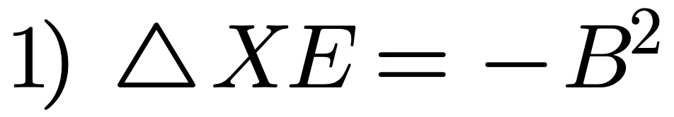
The principle of Faraday’s Law (equation 1) as detailed by most textbooks, is that an electric field can be related to the rate of change of a magnetic field. This electromagnetic feature can be expressed in a more elegant and informative way by reversing equation 1) to give that which is shown below as equation 3:
This is interpreted as a time varying magnetic flux, B² creating an electric field E such that the negative of the curl of the induced E field distribution is equal to the source B². The directive arrow is present in the relationship to indicate that the left-hand-side causes or creates the right-hand-side. The negative sign is a manifestation of Lenz’s law. In fact, the application of the reversed form of Faraday’s law is fully deployed in transformer theory, where a time varying magnetic flux creates, i.e., induces, a back EMF. Note that the E field in the reversed form of Faraday’s law is the induced E field from B’ and is not in anyway related to the independent electric field created from free charge through Gausse’s law.
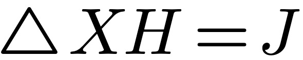
Consider now equation 2). In magnetostatics, it has always been accepted that current produces a magnetic field though the phenomenon called Ampere’s law. To get across the importance of this statement in a more meaningful physical and mathematical form, Ampere’s law should be expressed as Expression 5 below:

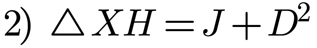
i.e., J (current density) creates a magnetic field H, such that the curl of H is equal to the source J. It is also known (though often ignored) that a magnetic field may be related to either a current as above or a time varying electric field. The latter source of magnetic field is sometimes referred to as the Maxwell Law, and may be expressed in the more informative form such as Equation 6 below:
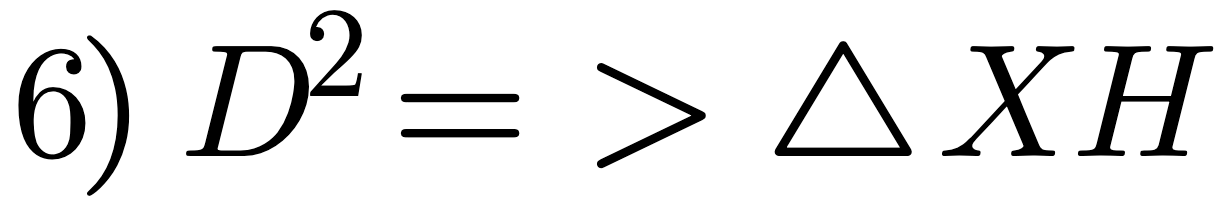
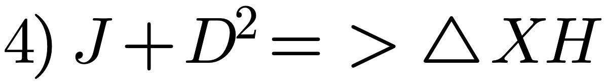
i.e., displacement current D’ (a time varying D field) creates a magnetic field H such that the curl of the H field distribution is equal to the source D’. We now see the importance of reversing equation 2) to give equation 4), i.e., J + D’ => D X H, which should now be interpreted as J + D’ or both can create a magnetic field H such that the curl of the H field distribution is equal to the source J + D’. The plus sign can, and should, be interpreted as analogous to the digital-logic OR symbol.
Unfortunately, many people fail to realize that an H field may, at any time, be the combination of two separately induced fields from independent types of sources, i.e., charge motion and displacement current.
The editor says we are out of space, so we will pick up here next month and apply what we have learned to create a magnetic field without running current thru a wire. This will be accomplished by a simple demonstration. That is essential to the process of building this type of Crossed-Field-Antenna. The heavy theory is behind us so it is down hill from here. Stay tuned.
Originally posted on the AntennaX Online Magazine by Maurice C. Hately, GM3HAT and Ted Hart, W5QJR
Last Updated : 20th March 2024